Session 4: Assignment explanation and answers

View datasets and create visualization.

# Import modules
from pyincore import FragilityService, IncoreClient, FragilityCurveSet, MappingSet, Dataset

from pyincore_viz.plotutil import PlotUtil as plot
from pyincore_viz.geoutil import GeoUtil as geoviz

# Connect to IN-CORE serivce by creating IncoreClient
client = IncoreClient()

Connection successful to IN-CORE services. pyIncore version detected: 0.9.3

# Exercise 1: 
# TODO: create a local dataset for building inventory with shapefiles ("sample_bldgs_w_guid.shp") 
#       and dataset inventory IN-CORE type: "ergo:buildingInventoryVer7"
# TODO: acquire GeoDataFrame object from the dataset


# Answer: 
# There is a shape file in your local directory. Sample building inventory has 4 files defining 
# the projection, attributes and other parts of a shape file (cpg, dbf, prj, shp, shx)

# use class method Dataset.from_file with path, filename and corresponding data type.
# Dataset.from_file(path, data_type)
bldgs = Dataset.from_file("sample_bldgs_w_guid.shp", data_type="ergo:buildingInventoryVer7")

# Object bldgs is now in pyincore object type. BTW pyIncore uses Fiona package to open shapefiles. 
print(type(bldgs))

# Construct GeoPanda's GeoDataFrame from a pyincore type.
# getting geodataframe of building dataset 
bldgs_gdf = bldgs.get_dataframe_from_shapefile()
print(type(bldgs_gdf))

# show first five rows only
bldgs_gdf.head()

<class 'pyincore.dataset.Dataset'>
<class 'geopandas.geodataframe.GeoDataFrame'>

	parid	struct_typ	year_built	no_stories	a_stories	b_stories	bsmt_type	sq_foot	gsq_foot	occ_type	...	archetype	appr_land	appr_tot	ffe_elev	g_elev	lhsm_elev	lon	lat	guid	geometry
0	018060 00010	C1	1978	1	1	0	NONE	6062	6062	COM6	...	12	None	None	None	None	None	-90.02585	35.14020	ac8b0b44-ae82-4c48-afb8-076e2d16c7e5	POINT (-90.02585 35.14020)
1	018060 00010	C1	1925	4	3	1	COMMERCIAL BSMT	19468	4867	COM6	...	12	None	None	None	None	None	-90.02585	35.14020	154b0a62-cae6-456d-8d90-635e3e1c2dcb	POINT (-90.02585 35.14020)
2	016001 00001C	S1	1924	14	13	1	COMMERCIAL BSMT	910583	65042	COM6	...	12	None	None	None	None	None	-90.01928	35.13640	9f9b11f8-c25c-4760-b1d2-a63bbeec8e72	POINT (-90.01928 35.13640)
3	012008 00012	URM	1910	5	3	2	COMMERCIAL BSMT	65112	13022	COM6	...	12	None	None	None	None	None	-90.07377	35.12344	28321416-e473-473b-ad0a-c3c38248acc7	POINT (-90.07377 35.12344)
4	001041 00001C	S1	1991	2	2	0	NONE	32094	16047	COM6	...	12	None	None	None	None	None	-90.04349	35.15360	b5069250-7a2b-47b1-9754-290528a6d72d	POINT (-90.04349 35.15360)

5 rows × 34 columns

# Exercise 2: 
# TODO: create a local dataset for building damage output with CSV ("memphis_eq_bldg_dmg_result.csv") - 
#       it should be in your browser if you ran session 4 notebook (dataset inventory IN-CORE type: "ergo:buildingDamageVer5")
# TODO: acquire DataFrame object from the dataset

# Answer: 
# A CSV file with guid, limit states and damage states is one of two resulting files of Infrastructure Damage Analyses 
# (building, pipeline etc.). The second, json file contains fragility ids, hazard values and other metadata 
# Locate CSV file in Jupyter browser directory

# Retrieve result dataset. If there is no csv file you need to run Building Damage Analyses from session 4 notebook.
bldgs = Dataset.from_file("memphis_eq_bldg_dmg_result.csv", data_type="ergo:buildingDamageVer5")

# Convert dataset to Pandas DataFrame
bldgs_df = bldgs.get_dataframe_from_csv()

print(type(bldgs_df))

# show first five rows only
bldgs_df.head()

<class 'pandas.core.frame.DataFrame'>

	guid	LS_0	LS_1	LS_2	DS_0	DS_1	DS_2	DS_3
0	ac8b0b44-ae82-4c48-afb8-076e2d16c7e5	0.848149	0.327322	2.722964e-02	0.151851	0.520827	0.300092	2.722964e-02
1	154b0a62-cae6-456d-8d90-635e3e1c2dcb	0.844343	0.328299	2.860543e-02	0.155657	0.516043	0.299694	2.860543e-02
2	9f9b11f8-c25c-4760-b1d2-a63bbeec8e72	0.896774	0.480925	8.756720e-02	0.103226	0.415849	0.393358	8.756720e-02
3	28321416-e473-473b-ad0a-c3c38248acc7	0.828098	0.293753	2.738378e-02	0.171902	0.534345	0.266369	2.738378e-02
4	b5069250-7a2b-47b1-9754-290528a6d72d	0.970343	0.154677	1.000000e-10	0.029657	0.815666	0.154677	1.000000e-10

# Exercise 3: 
# TODO: Join/merge building inventory GeoDataframe and damage output Dataframe using results of Excercise 1 and 2.

# Answer: 
# We now have two objects, Geopanda's GeoDataFrame with buildings attributes and coordinates 
# and Panda's DataFrame with  Damage states. Both objects have GUID referencing buildings.

# Merge/join two dataframe using GUID. We can also specify first three columns, guid, struct_typ and geometry, 
# and their order.
bldgs_joined_gdf = bldgs_gdf[['guid', 'struct_typ', 'geometry', 'appr_bldg']].merge(bldgs_df, on='guid')
bldgs_joined_gdf.head()

	guid	struct_typ	geometry	appr_bldg	LS_0	LS_1	LS_2	DS_0	DS_1	DS_2	DS_3
0	ac8b0b44-ae82-4c48-afb8-076e2d16c7e5	C1	POINT (-90.02585 35.14020)	163315	0.848149	0.327322	2.722964e-02	0.151851	0.520827	0.300092	2.722964e-02
1	154b0a62-cae6-456d-8d90-635e3e1c2dcb	C1	POINT (-90.02585 35.14020)	524485	0.844343	0.328299	2.860543e-02	0.155657	0.516043	0.299694	2.860543e-02
2	9f9b11f8-c25c-4760-b1d2-a63bbeec8e72	S1	POINT (-90.01928 35.13640)	49457042	0.896774	0.480925	8.756720e-02	0.103226	0.415849	0.393358	8.756720e-02
3	28321416-e473-473b-ad0a-c3c38248acc7	URM	POINT (-90.07377 35.12344)	367311	0.828098	0.293753	2.738378e-02	0.171902	0.534345	0.266369	2.738378e-02
4	b5069250-7a2b-47b1-9754-290528a6d72d	S1	POINT (-90.04349 35.15360)	1027399	0.970343	0.154677	1.000000e-10	0.029657	0.815666	0.154677	1.000000e-10

# Exercise 4: 
# TODO: Using joined GeoDataFrame, display the table grouped by "struct_type" and show a sum of apprasial 
#       value of buildings "appr_bldg" 

# Answer: 
# We have a joined object, GeoDataFrame bldgs_joined_gdf with all attributes (columns). We can show only guid
# and struct_type and appr_bldg columns. Dont forget to keep geometry column or new dataframe 
# will not be georeferenced

bldgs_new = bldgs_joined_gdf[['guid', 'geometry', 'struct_typ', 'appr_bldg']]
bldgs_new.head()

	guid	geometry	struct_typ	appr_bldg
0	ac8b0b44-ae82-4c48-afb8-076e2d16c7e5	POINT (-90.02585 35.14020)	C1	163315
1	154b0a62-cae6-456d-8d90-635e3e1c2dcb	POINT (-90.02585 35.14020)	C1	524485
2	9f9b11f8-c25c-4760-b1d2-a63bbeec8e72	POINT (-90.01928 35.13640)	S1	49457042
3	28321416-e473-473b-ad0a-c3c38248acc7	POINT (-90.07377 35.12344)	URM	367311
4	b5069250-7a2b-47b1-9754-290528a6d72d	POINT (-90.04349 35.15360)	S1	1027399

# Exercise 4 cont.:

# Run stastics on a column.
# Sum of all rows = 270,160,346
total = bldgs_new["appr_bldg"].sum()
print(total)

270160346

# Exercise 4 cont.:

# Run stastics on a column (first five rows).
# Sum of 5 rows = 51,539,552 with mean value of 10,307,910
bldgs_new["appr_bldg"].head().describe()

count    5.000000e+00
mean     1.030791e+07
std      2.188736e+07
min      1.633150e+05
25%      3.673110e+05
50%      5.244850e+05
75%      1.027399e+06
max      4.945704e+07
Name: appr_bldg, dtype: float64

# Exercise 5: 
# TODO: Using joined GeoDataFrame, plot a pie chart of (DS_0, DS_1, DS_2, DS_3) with a building with highest 
#       value of DS_3

# Answer: 
# We have a joined object, GeoDataFrame bldgs_joined_gdf with all attributes (columns). We can create a new one
# only with guid and damage states probability values.
df_ds = bldgs_joined_gdf[['guid', 'DS_0', 'DS_1', 'DS_2', 'DS_3']]
df_ds.head()

	guid	DS_0	DS_1	DS_2	DS_3
0	ac8b0b44-ae82-4c48-afb8-076e2d16c7e5	0.151851	0.520827	0.300092	2.722964e-02
1	154b0a62-cae6-456d-8d90-635e3e1c2dcb	0.155657	0.516043	0.299694	2.860543e-02
2	9f9b11f8-c25c-4760-b1d2-a63bbeec8e72	0.103226	0.415849	0.393358	8.756720e-02
3	28321416-e473-473b-ad0a-c3c38248acc7	0.171902	0.534345	0.266369	2.738378e-02
4	b5069250-7a2b-47b1-9754-290528a6d72d	0.029657	0.815666	0.154677	1.000000e-10

# Exercise 5 cont: 
# Return the entire row with max value of DS_3 column
df = df_ds[df_ds['DS_3']==df_ds['DS_3'].max()]
df.head()

	guid	DS_0	DS_1	DS_2	DS_3
14	6dd342ef-498c-43a9-85cd-35ad76e4c279	0.143819	0.409244	0.352468	0.094468

# Exercise 5 cont: 

# We use Panda's plot method for pie chart visualization of our four DS probabilities.
# First, the dataframe must be transposed to get rows of DS
df_pie = df[['DS_0', 'DS_1', 'DS_2', 'DS_3']].transpose()
# Rename the column for proper legend
df_pie.columns = ['probability']
df_pie.head()

	probability
DS_0	0.143819
DS_1	0.409244
DS_2	0.352468
DS_3	0.094468

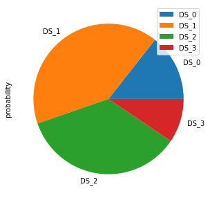
# Exercise 5 cont: 

# Create pie chart
plot = df_pie.plot.pie(subplots=True, figsize=(5, 5))

# Exercise 6: 
# TODO: Using joined GeoDataFrame, display a table of buidings with DS_3 >= 0.05 and sorted by DS_3

# Answer: 
# We have our joined object, GeoDataFrame bldgs_joined_gdf with all attributes (columns). We can create 
# a new one only with guid and damage states probability values:
# df_ds = bldgs_joined_gdf[['guid', 'DS_0', 'DS_1', 'DS_2', 'DS_3']]
# or re-use df_ds object from Exercise 5

df_ds3 = df_ds[df_ds['DS_3']>=0.05]
df_ds3.sort_values(by=['DS_3'])

	guid	DS_0	DS_1	DS_2	DS_3
6	11395729-3727-449d-9848-778d68edd7d8	0.076171	0.432794	0.420815	0.070220
11	d7603d04-6917-478c-8bb7-50cf9118f973	0.119953	0.434135	0.371550	0.074362
2	9f9b11f8-c25c-4760-b1d2-a63bbeec8e72	0.103226	0.415849	0.393358	0.087567
14	6dd342ef-498c-43a9-85cd-35ad76e4c279	0.143819	0.409244	0.352468	0.094468

# Exercise 7: 
# TODO: Using joined GeoDataFrame, plot a map of buidings with DS_3 >= 0.05 and sorted by DS_3

# Answer: 
# We have sorted object, df_ds3 from Exercise 6 however we removed the geometry. We need to go back and use 
# georeferenced object bldgs_joined_gdf with guid, geometry and DS_3.

bldgs_ds3 = bldgs_joined_gdf[['guid', 'geometry', 'DS_3']]
bldgs_ds3.head()

	guid	geometry	DS_3
0	ac8b0b44-ae82-4c48-afb8-076e2d16c7e5	POINT (-90.02585 35.14020)	2.722964e-02
1	154b0a62-cae6-456d-8d90-635e3e1c2dcb	POINT (-90.02585 35.14020)	2.860543e-02
2	9f9b11f8-c25c-4760-b1d2-a63bbeec8e72	POINT (-90.01928 35.13640)	8.756720e-02
3	28321416-e473-473b-ad0a-c3c38248acc7	POINT (-90.07377 35.12344)	2.738378e-02
4	b5069250-7a2b-47b1-9754-290528a6d72d	POINT (-90.04349 35.15360)	1.000000e-10

# Exercise 7 cont: 

# We filter buildings by DS_3 value and sort them:
ds3 = bldgs_ds3[bldgs_ds3['DS_3']>=0.05]
ds3_sorted = ds3.sort_values(by=['DS_3'])
ds3_sorted.head()

	guid	geometry	DS_3
6	11395729-3727-449d-9848-778d68edd7d8	POINT (-90.04349 35.15360)	0.070220
11	d7603d04-6917-478c-8bb7-50cf9118f973	POINT (-89.86438 35.09755)	0.074362
2	9f9b11f8-c25c-4760-b1d2-a63bbeec8e72	POINT (-90.01928 35.13640)	0.087567
14	6dd342ef-498c-43a9-85cd-35ad76e4c279	POINT (-89.77456 35.20624)	0.094468

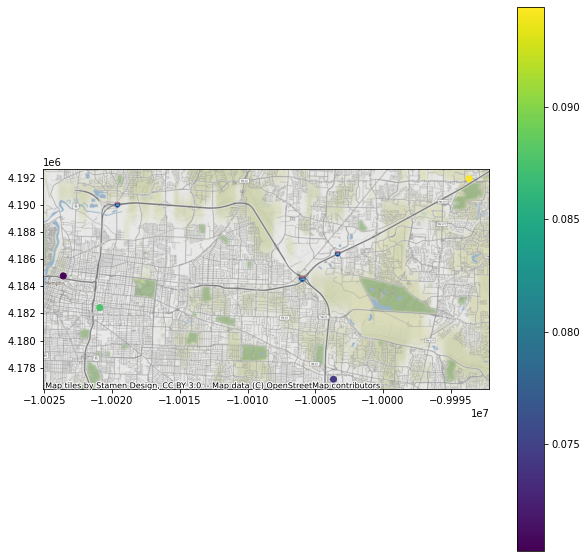
# Exercise 7 cont: 

# Plot a map of ds3_sorted GeoPandasDataset with pyincore_viz
geoviz.plot_gdf_map(ds3_sorted, 'DS_3', basemap=True)